Integral merupakan kebalikan derivatif.
Definisi
Misalkan kita mempunyai fungsi kecepatan terhadap waktu
v ( t ) = t 2 v(t) = t^2
v ( t ) = t 2
Kita disuruh mencari fungsi yang menunjukkan jarak yang ditempuh pada waktu tertentu. Kita tidak bisa mencarinya dengan s = v t s=vt s = v t v v v v v v v ( t ) v(t) v ( t ) s = v t s=vt s = v t v v v v v v
v = d s d t → d s d t = t 2 v ={ds \over dt} \rightarrow {ds \over dt} = t^2
v = d t d s → d t d s = t 2
Untuk mencari fungsi s s s t 2 t^2 t 2
s = t 3 → d s d t = 3 t 2 s = 1 3 t 3 → d s d t = t 2 \begin{align*}
s &= t^3 &\rightarrow {ds \over dt} &= 3t^2\\
s &= {1 \over 3}t^3 &\rightarrow {ds \over dt} &= t^2\\
\end{align*}
s s = t 3 = 3 1 t 3 → d t d s → d t d s = 3 t 2 = t 2
Maka fungsi yang memenuhi adalah s ( t ) = 1 3 t 3 s(t) = {1 \over 3}t^3 s ( t ) = 3 1 t 3
s = 1 3 t 3 + 1 → d s d t = t 2 s = 1 3 t 3 + 20 → d s d t = t 2 \begin{align*}
s &= {1 \over 3}t^3 + 1 &\rightarrow {ds \over dt} &= t^2\\
s &= {1 \over 3}t^3 + 20 &\rightarrow {ds \over dt} &= t^2\\
\end{align*}
s s = 3 1 t 3 + 1 = 3 1 t 3 + 20 → d t d s → d t d s = t 2 = t 2
Maka fungsi yang memenuhi adalah s ( t ) = 1 3 t 3 + c s(t) = {1 \over 3}t^3 + c s ( t ) = 3 1 t 3 + c c c c c c c t = 0 t=0 t = 0 1 3 t 3 + c {1 \over 3}t^3 + c 3 1 t 3 + c t 2 t^2 t 2
s = ∫ v d t = ∫ t 2 d t = 1 3 t 3 + c s = \int v dt = \int t^2 dt = {1 \over 3}t^3 + c
s = ∫ v d t = ∫ t 2 d t = 3 1 t 3 + c
Hubungannya dengan derivatif:
v = d s d t = t 2 v = {ds \over dt} = t^2
v = d t d s = t 2
Lalu apa hubungan integral dengan luas area dibawah kurva?. Misalkan kita menggambar fungsi v ( t ) v(t) v ( t )
t t t t t t d t dt d t d s ds d s d t dt d t d s = v ( t ) d t ds = v(t)dt d s = v ( t ) d t
v ( t ) = d s d t → s = ∫ v ( t ) d t v(t)={ds \over dt} \rightarrow s = \int v(t) dt
v ( t ) = d t d s → s = ∫ v ( t ) d t
Jadi integral menunjukkan luas area dibawah fungsi/kurva. d s ds d s s s s
Integral tak tentu (antiderivatif) menunjukkan luas daerah di bawah suatu kurva. Integral tak tentu dilambangkan dengan:
F ( x ) = ∫ f ( x ) d x F(x) = \int f(x) dx
F ( x ) = ∫ f ( x ) d x
maka
d F d x = f ( x ) {dF \over dx} = f(x)
d x d F = f ( x )
Lalu bagaimana jika suatu kurva berada di bawah sumbu x. Kita bisa menggambar fungsi f ( x ) = sin ( x ) f(x)=\sin(x) f ( x ) = sin ( x ) F ( x ) = ∫ sin ( x ) d x F(x) = \int \sin(x)dx F ( x ) = ∫ sin ( x ) d x
Pada x x x f ( x ) d x f(x)dx f ( x ) d x f ( x ) f(x) f ( x ) f ( x ) d x = d F f(x)dx=dF f ( x ) d x = d F → \rightarrow → d F d x = f ( x ) {dF \over dx} = f(x) d x d F = f ( x ) → \rightarrow → F ( x ) = ∫ f ( x ) d x F(x) = \int f(x) dx F ( x ) = ∫ f ( x ) d x
Apakah ada cara untuk menghitung luas yang ditutupi kurva dan dibatasi dua nilai. Kita bisa mencobanya dengan menggambar fungsi f ( x ) f(x) f ( x )
Luas daerah yang dibatasi oleh 0 dan x 0 x_0 x 0 F ( x 0 ) F(x_0) F ( x 0 ) x 1 x_1 x 1 F ( x 1 ) F(x_1) F ( x 1 ) x 0 x_0 x 0 x 1 x_1 x 1 x 1 x_1 x 1 x 0 x_0 x 0
L = F ( x 1 ) − F ( x 0 ) L = F(x_1) - F(x_0)
L = F ( x 1 ) − F ( x 0 )
Luas daerah tersebut disebut sebagai integral tentu yang dibatasi oleh x 0 x_0 x 0 x 1 x_1 x 1
∫ x 0 x 1 f ( x ) d x = F ( x 1 ) − F ( x 0 ) \int_{x_0}^{x_1}f(x)dx = F(x_1) - F(x_0)
∫ x 0 x 1 f ( x ) d x = F ( x 1 ) − F ( x 0 )
Integral tentu menunjukkan daerah yang ditutupi kurva dan dibatasi oleh dua nilai. Integral tentu f ( x ) f(x) f ( x ) a a a b b b
∫ a b f ( x ) d x = F ( b ) − F ( a ) \int_a^b f(x) dx = F(b) - F(a)
∫ a b f ( x ) d x = F ( b ) − F ( a )
a a a b b b
d F d x = f ( x ) {dF \over dx} = f(x)
d x d F = f ( x )
atau
F ′ ( x ) = f ( x ) F'(x) = f(x)
F ′ ( x ) = f ( x )
Aturan Pangkat
Kita akan menggunakan sifat derivatif untuk mencari tahu sifat ini
d d x ( x n + c ) = n x n − 1 ↓ ∫ n x n − 1 = x n + c d d x ( x n n + c ) = 1 n n x n − 1 ↓ d d x ( x n n + c ) = x n − 1 ↓ ∫ x n − 1 = x n n + c \begin{gather*}
{d \over dx}\left(x^n + c\right)= nx^{n-1}\\
\downarrow\\
\int nx^{n-1} = x^n + c\\
\\
\\
{d \over dx}\left({x^n \over n} + c\right)= {1 \over n} nx^{n-1}\\
\downarrow\\
{d \over dx}\left({x^n \over n} + c\right)= x^{n-1}\\
\downarrow\\
\int x^{n-1} = {x^n \over n} + c
\end{gather*}
d x d ( x n + c ) = n x n − 1 ↓ ∫ n x n − 1 = x n + c d x d ( n x n + c ) = n 1 n x n − 1 ↓ d x d ( n x n + c ) = x n − 1 ↓ ∫ x n − 1 = n x n + c
Misalkan m = n − 1 m=n-1 m = n − 1 → \rightarrow → n = m + 1 n=m+1 n = m + 1
∫ x n − 1 = x n n + c ∫ x m = x m + 1 m + 1 + c \begin{align*}
\int x^{n-1} &= {x^n \over n} + c \\
\int x^m &= {x^{m+1} \over m+1} + c \\
\end{align*}
∫ x n − 1 ∫ x m = n x n + c = m + 1 x m + 1 + c
Aturan pangkat pada integral
∫ x n = x n + 1 n + 1 + c \int x^n = {x^{n+1} \over n+1} + c
∫ x n = n + 1 x n + 1 + c
Integral dari Konstanta
Menurut derivatif. a = a = a =
d d x ( x + c ) = 1 ↓ ∫ 1 d x = x + c ↓ ∫ d x = x + c d d x ( a x + c ) = a ↓ ∫ a d x = a x + c \begin{gather*}
{d \over dx}(x + c)=1\\
\downarrow\\
\int 1 dx = x + c\\
\downarrow\\
\int dx = x + c\\
\\
\\
{d \over dx}(ax + c)=a\\
\downarrow\\
\int a dx = ax + c
\end{gather*}
d x d ( x + c ) = 1 ↓ ∫ 1 d x = x + c ↓ ∫ d x = x + c d x d ( a x + c ) = a ↓ ∫ a d x = a x + c
Misalkan a = a = a = ∫ a d x = a x + c \int adx = ax + c ∫ a d x = a x + c a = 1 a=1 a = 1 a a a ∫ d x = x + c \int dx = x + c ∫ d x = x + c
Perkalian dengan Konstanta
Menurut derivatif. a = a = a = f ( x ) = f(x)= f ( x ) =
d d x ( a F ( x ) + c ) = ( a d F d x ) ↓ ∫ ( a d F d x ) d x = a F ( x ) + c \begin{gather*}
{d \over dx}(aF(x) + c) = \left(a{dF \over dx}\right)\\
\downarrow\\
\int \left(a{dF \over dx}\right)dx = aF(x) + c
\end{gather*}
d x d ( a F ( x ) + c ) = ( a d x d F ) ↓ ∫ ( a d x d F ) d x = a F ( x ) + c
Misalkan:
d F d x = f ( x ) ↓ ∫ f ( x ) d x = F ( x ) \begin{gather*}
{dF \over dx} = f(x)\\
\downarrow\\
\int f(x)dx = F(x)
\end{gather*}
d x d F = f ( x ) ↓ ∫ f ( x ) d x = F ( x )
Maka:
∫ ( a d F d x ) d x = a F ( x ) + c ↓ ∫ a f ( x ) d x = a ∫ f ( x ) d x + c \begin{gather*}
\int \left(a{dF \over dx}\right)dx = aF(x) + c\\
\downarrow\\
\int af(x)dx = a\int f(x)dx + c
\end{gather*}
∫ ( a d x d F ) d x = a F ( x ) + c ↓ ∫ a f ( x ) d x = a ∫ f ( x ) d x + c
Menurut intuisi. Saat kita mengalikan suatu fungsi dengan konstanta misalknya 3. Maka nilai y y y
∫ 3 f ( x ) d x = 3 ∫ f ( x ) d x \int 3f(x)dx = 3 \int f(x)dx
∫ 3 f ( x ) d x = 3 ∫ f ( x ) d x
Ini juga berlaku saat fungsi dikalikan konstanta lain:
∫ a f ( x ) d x = a ∫ f ( x ) d x \int af(x)dx = a \int f(x)dx
∫ a f ( x ) d x = a ∫ f ( x ) d x
Perkalian dengan konstanta pada integral:
∫ a f ( x ) d x = a ∫ f ( x ) d x \int af(x)dx = a \int f(x)dx ∫ a f ( x ) d x = a ∫ f ( x ) d x
Sifat Penjumlahan dan Pengurangan
Secara intuisi, jika kita menjumlahkan dua fungsi. Maka nilai y-nya merupakan penjumlahan nilai kedua fungsi. Sehingga luas daerah di bawah kurva juga merupakan penjumlahan luas daerah dari kedua fungsi.
∫ f ( x ) + g ( x ) d x = ∫ f ( x ) d x + ∫ g ( x ) d x \int f(x) + g(x)dx = \int f(x)dx + \int g(x)dx
∫ f ( x ) + g ( x ) d x = ∫ f ( x ) d x + ∫ g ( x ) d x
Begitu juga dengan pengurangan:
∫ f ( x ) − g ( x ) d x = ∫ f ( x ) d x − ∫ g ( x ) d x \int f(x) - g(x)dx = \int f(x)dx - \int g(x)dx
∫ f ( x ) − g ( x ) d x = ∫ f ( x ) d x − ∫ g ( x ) d x
Bukti menggunakan turunan:
Misal:
d F d x = f ( x ) → ∫ f ( x ) d x = F ( x ) d G d x = g ( x ) → ∫ g ( x ) d x = G ( x ) \begin{align*}
{dF \over dx} = f(x) &\rightarrow \int f(x)dx = F(x)\\
{dG \over dx} = g(x) &\rightarrow \int g(x)dx = G(x)\\
\end{align*}
d x d F = f ( x ) d x d G = g ( x ) → ∫ f ( x ) d x = F ( x ) → ∫ g ( x ) d x = G ( x )
Maka:
d ( F ( x ) + G ( x ) ) d x = d F d x + d G d x ↓ ∫ ( d F d x + d G d x ) d x = F ( x ) + G ( x ) ↓ ∫ ( f ( x ) + g ( x ) ) d x = ∫ f ( x ) d x + ∫ g ( x ) d x \begin{gather*}
{d(F(x) + G(x)) \over dx} = {dF \over dx} + {dG \over dx}\\
\downarrow\\
\int \left( {dF \over dx} + {dG \over dx} \right) dx = F(x) + G(x)\\
\downarrow\\
\int \left( f(x) + g(x) \right) dx = \int f(x)dx + \int g(x)dx\\
\end{gather*}
d x d ( F ( x ) + G ( x )) = d x d F + d x d G ↓ ∫ ( d x d F + d x d G ) d x = F ( x ) + G ( x ) ↓ ∫ ( f ( x ) + g ( x ) ) d x = ∫ f ( x ) d x + ∫ g ( x ) d x
d ( F ( x ) − G ( x ) ) d x = d F d x − d G d x ↓ ∫ ( d F d x − d G d x ) d x = F ( x ) − G ( x ) ↓ ∫ ( f ( x ) − g ( x ) ) d x = ∫ f ( x ) d x − ∫ g ( x ) d x \begin{gather*}
{d(F(x) - G(x)) \over dx} = {dF \over dx} - {dG \over dx}\\
\downarrow\\
\int \left( {dF \over dx} - {dG \over dx} \right) dx = F(x) - G(x)\\
\downarrow\\
\int \left( f(x) - g(x) \right) dx = \int f(x)dx - \int g(x)dx\\
\end{gather*}
d x d ( F ( x ) − G ( x )) = d x d F − d x d G ↓ ∫ ( d x d F − d x d G ) d x = F ( x ) − G ( x ) ↓ ∫ ( f ( x ) − g ( x ) ) d x = ∫ f ( x ) d x − ∫ g ( x ) d x
Penjumlahan dan pengurangan pada integral
∫ ( f ( x ) + g ( x ) ) d x = ∫ f ( x ) d x + ∫ g ( x ) d x ∫ ( f ( x ) − g ( x ) ) d x = ∫ f ( x ) d x − ∫ g ( x ) d x \begin{align*}
\int \left( f(x) + g(x) \right) dx &= \int f(x)dx + \int g(x)dx\\
\int \left( f(x) - g(x) \right) dx &= \int f(x)dx - \int g(x)dx
\end{align*}
∫ ( f ( x ) + g ( x ) ) d x ∫ ( f ( x ) − g ( x ) ) d x = ∫ f ( x ) d x + ∫ g ( x ) d x = ∫ f ( x ) d x − ∫ g ( x ) d x
Subtitusi u (u-sub)
Teknik ini merupakan kebalikan dari aturan rantai pada turunan.
d F d x = f ( x ) ↓ ∫ f ( x ) d x = F ( x ) d ( F ( G ( x ) ) ) d ( G ( x ) ) = f ( G ( x ) ) ↓ ∫ f ( G ( x ) ) d ( G ( x ) ) = F ( G ( x ) ) d G d x = g ( x ) ↓ ∫ g ( x ) d x = G ( x ) d d x ( F ( G ( x ) ) ) = d ( F ( G ( x ) ) ) d ( G ( x ) ) ⋅ d G d x ↓ ∫ d ( F ( G ( x ) ) ) d ( G ( x ) ) ⋅ d G d x d x = F ( G ( x ) ) ↓ ∫ f ( G ( x ) ) ⋅ g ( x ) d x = ∫ f ( G ( x ) ) d ( G ( x ) ) \begin{gather*}
{dF \over dx} = f(x)\\
\downarrow\\
\int f(x)dx = F(x)\\
\\
\\
{d(F(G(x))) \over d(G(x))} = f(G(x))\\
\downarrow\\
\int f(G(x))d(G(x)) = F(G(x))\\
\\
\\
{dG \over dx} = g(x)\\
\downarrow\\
\int g(x)dx = G(x)
\\
\\
{d \over dx}\left( F(G(x))\right) = {d(F(G(x))) \over d(G(x))} \cdot {dG \over dx}\\
\downarrow\\
\int {d(F(G(x))) \over d(G(x))} \cdot {dG \over dx}dx = F(G(x))\\
\downarrow\\
\int f(G(x))\cdot g(x)dx = \int f(G(x))d(G(x))\\
\end{gather*}
d x d F = f ( x ) ↓ ∫ f ( x ) d x = F ( x ) d ( G ( x )) d ( F ( G ( x ))) = f ( G ( x )) ↓ ∫ f ( G ( x )) d ( G ( x )) = F ( G ( x )) d x d G = g ( x ) ↓ ∫ g ( x ) d x = G ( x ) d x d ( F ( G ( x )) ) = d ( G ( x )) d ( F ( G ( x ))) ⋅ d x d G ↓ ∫ d ( G ( x )) d ( F ( G ( x ))) ⋅ d x d G d x = F ( G ( x )) ↓ ∫ f ( G ( x )) ⋅ g ( x ) d x = ∫ f ( G ( x )) d ( G ( x ))
Agar lebih sederhana kita misalkan u = G ( x ) u=G(x) u = G ( x ) u ′ = g ( x ) u' = g(x) u ′ = g ( x )
∫ f ( u ) ⋅ u ′ d x = ∫ f ( u ) d u \int f(u)\cdot u'dx = \int f(u)du
∫ f ( u ) ⋅ u ′ d x = ∫ f ( u ) d u
Pada Integral tentu berlaku aturan khusus yaitu perubahan batas:
∫ f ( G ( x ) ) d ( G ( x ) ) = F ( G ( x ) ) ↓ ∫ a b f ( G ( x ) ) d ( G ( x ) ) = F ( b ) − F ( a ) ↓ ∫ G ( a ) G ( b ) f ( G ( x ) ) d ( G ( x ) ) = F ( G ( b ) ) − F ( g ( a ) ) \begin{gather*}
\int f(G(x))d(G(x)) = F(G(x))\\
\downarrow\\
\int_a^b f(G(x))d(G(x)) = F(b) - F(a)\\
\downarrow\\
\int_{G(a)}^{G(b)} f(G(x))d(G(x)) = F(G(b)) - F(g(a))
\end{gather*}
∫ f ( G ( x )) d ( G ( x )) = F ( G ( x )) ↓ ∫ a b f ( G ( x )) d ( G ( x )) = F ( b ) − F ( a ) ↓ ∫ G ( a ) G ( b ) f ( G ( x )) d ( G ( x )) = F ( G ( b )) − F ( g ( a ))
Mengapa perubahan dari baris 1 ke 2 bisa begitu?∫ a b \int_a^b ∫ a b d x dx d x x x x a a a b b b d ( G ( x ) ) d(G(x)) d ( G ( x )) G ( x ) G(x) G ( x ) G ( x ) G(x) G ( x ) a a a b b b
∫ f ( x ) d x = F ( x ) ↓ ∫ a b f ( x ) d x = F ( b ) − F ( a ) ↓ ∫ a b f ( G ( x ) ) d ( G ( x ) ) = F ( b ) − F ( a ) \begin{gather*}
\int f(x)dx = F(x)\\
\downarrow\\
\int_a^b f(x)dx = F(b) - F(a)\\
\downarrow\\
\int_a^b f(G(x))d(G(x)) = F(b) - F(a)
\end{gather*}
∫ f ( x ) d x = F ( x ) ↓ ∫ a b f ( x ) d x = F ( b ) − F ( a ) ↓ ∫ a b f ( G ( x )) d ( G ( x )) = F ( b ) − F ( a )
∫ d ( F ( G ( x ) ) ) d ( G ( x ) ) ⋅ d G d x d x = F ( G ( x ) ) ↓ ∫ a b d ( F ( G ( x ) ) ) d ( G ( x ) ) ⋅ d G d x d x = F ( G ( b ) ) − F ( G ( a ) ) ↓ ∫ a b f ( G ( x ) ) ⋅ g ( x ) d x = F ( G ( b ) ) − F ( G ( a ) ) ↓ ∫ a b f ( G ( x ) ) ⋅ g ( x ) d x = ∫ G ( a ) G ( b ) f ( G ( x ) ) d ( G ( x ) ) ↓ ∫ a b f ( u ) ⋅ u ′ d x = ∫ u ( a ) u ( b ) f ( u ) d u \begin{gather*}
\\
\\
\int {d(F(G(x))) \over d(G(x))} \cdot {dG \over dx}dx = F(G(x))\\
\downarrow\\
\int_a^b {d(F(G(x))) \over d(G(x))} \cdot {dG \over dx}dx = F(G(b)) - F(G(a)) \\
\downarrow\\
\int_a^b f(G(x))\cdot g(x)dx = F(G(b)) - F(G(a))\\
\downarrow\\
\int_a^b f(G(x))\cdot g(x)dx = \int_{G(a)}^{G(b)} f(G(x))d(G(x))\\
\downarrow\\
\int_a^b f(u)\cdot u'dx = \int_{u(a)}^{u(b)} f(u)du\\
\end{gather*}
∫ d ( G ( x )) d ( F ( G ( x ))) ⋅ d x d G d x = F ( G ( x )) ↓ ∫ a b d ( G ( x )) d ( F ( G ( x ))) ⋅ d x d G d x = F ( G ( b )) − F ( G ( a )) ↓ ∫ a b f ( G ( x )) ⋅ g ( x ) d x = F ( G ( b )) − F ( G ( a )) ↓ ∫ a b f ( G ( x )) ⋅ g ( x ) d x = ∫ G ( a ) G ( b ) f ( G ( x )) d ( G ( x )) ↓ ∫ a b f ( u ) ⋅ u ′ d x = ∫ u ( a ) u ( b ) f ( u ) d u
Teknik subtitusi merupakan teknik pada integral. Kita harus memilih u u u d u du d u ∫ f ( u ) ⋅ u ′ d x = ∫ f ( u ) d u \int f(u)\cdot u'dx = \int f(u)du ∫ f ( u ) ⋅ u ′ d x = ∫ f ( u ) d u ∫ a b f ( u ) ⋅ u ′ d x = ∫ u ( a ) u ( b ) f ( u ) d u \int_a^b f(u)\cdot u'dx = \int_{u(a)}^{u(b)} f(u)du ∫ a b f ( u ) ⋅ u ′ d x = ∫ u ( a ) u ( b ) f ( u ) d u
Contoh: ∫ 0 2 2 5 − 2 x d x \int_{0}^{2} 2\sqrt{5-2x} dx ∫ 0 2 2 5 − 2 x d x
u = 5 − 2 x u ( 0 ) = 5 − 0 = 5 u ( 1 ) = 5 − 2 ⋅ 2 = 1 d u d x = − 2 d x = − d u 2 ∫ 0 2 2 5 − 2 x d x = ∫ 5 1 2 u ⋅ − d u 2 = − ∫ 5 1 u 1 2 d u = − ( 2 3 u 3 2 ) ∣ 5 1 = − 2 3 ( 1 3 2 − 5 3 2 ) = 2 3 ( 5 3 2 − 1 ) = 2 3 ( 5 3 − 1 ) = 2 3 ( 5 2 5 − 1 ) = 2 3 ( 5 5 − 1 ) \begin{aligned}
u & =5-2x\\
u( 0) & =5-0\\
& =5\\
u( 1) & =5-2\cdot 2\\
& =1\\
\frac{du}{dx} & =-2\\
dx & =\frac{-du}{2}\\
\int_{0}^{2} 2\sqrt{5-2x} dx & =\int _{5}^{1} 2\sqrt{u} \cdot \frac{-du}{2}\\
& =-\int _{5}^{1} u^{\frac{1}{2}} du\\
& =-\left(\frac{2}{3} u^{\frac{3}{2}}\right)\Bigl|_{5}^{1}\\
& =-\frac{2}{3}\left( 1^{\frac{3}{2}} -5^{\frac{3}{2}}\right)\\
& =\frac{2}{3}\left( 5^{\frac{3}{2}} -1\right)\\
& =\frac{2}{3}\left(\sqrt{5^{3}} -1\right)\\
& =\frac{2}{3}\left(\sqrt{5^{2} 5} -1\right)\\
& =\frac{2}{3}\left( 5\sqrt{5} -1\right)
\end{aligned}
u u ( 0 ) u ( 1 ) d x d u d x ∫ 0 2 2 5 − 2 x d x = 5 − 2 x = 5 − 0 = 5 = 5 − 2 ⋅ 2 = 1 = − 2 = 2 − d u = ∫ 5 1 2 u ⋅ 2 − d u = − ∫ 5 1 u 2 1 d u = − ( 3 2 u 2 3 ) 5 1 = − 3 2 ( 1 2 3 − 5 2 3 ) = 3 2 ( 5 2 3 − 1 ) = 3 2 ( 5 3 − 1 ) = 3 2 ( 5 2 5 − 1 ) = 3 2 ( 5 5 − 1 )
Hubungan integral tak tentu dengan integral tentu
Seharusnya ada hubungan dari dua integral tersebut
d F d x = f ( x ) → ∫ f ( x ) d x = F ( x ) → ∫ a b f ( x ) d x = F ( b ) − F ( a ) \begin{align*}
{dF \over dx} = f(x) &\rightarrow \int f(x)dx = F(x)\\
&\rightarrow \int_a^b f(x)dx = F(b) - F(a)
\end{align*}
d x d F = f ( x ) → ∫ f ( x ) d x = F ( x ) → ∫ a b f ( x ) d x = F ( b ) − F ( a )
∫ a b f ( x ) d x = ( ∫ f ( x ) d x ) ( b ) − ( ∫ f ( x ) d x ) ( a ) = ( ∫ f ( x ) d x ) ∣ a b F ( x ) ∣ a b = F ( b ) − F ( a ) \begin{align*}
\int_a^b f(x)dx &= \left(\int f(x)dx\right)(b) - \left(\int f(x)dx\right)(a)\\
&= \left(\int f(x)dx\right) \Big|_a^b\\
F(x)\Big|_a^b &= F(b) - F(a)
\end{align*}
∫ a b f ( x ) d x F ( x ) a b = ( ∫ f ( x ) d x ) ( b ) − ( ∫ f ( x ) d x ) ( a ) = ( ∫ f ( x ) d x ) a b = F ( b ) − F ( a )
Maksud yang harus berhati hati adalah notasi ∣ a b \Big|_a^b a b
Mengintegrasikan ∫ 0 2 2 5 − 2 x d x \int_{0}^{2} 2\sqrt{5-2x} dx ∫ 0 2 2 5 − 2 x d x
u = 5 − 2 x d u d x = − 2 d x = − d u 2 ∫ 0 2 2 5 − 2 x d x = ( ∫ 2 5 − 2 x d x ) ∣ 0 2 = ( ∫ 2 u ⋅ − d u 2 ) ∣ 0 2 = ( ∫ − u 1 2 d u ) ∣ 0 2 = ( − 2 3 u 3 2 ) ∣ 0 2 = − 2 3 ( 2 3 2 − 0 3 2 ) = − 2 3 ( 2 3 2 ) = − 2 3 ( 2 3 ) = − 2 3 ( 2 2 ) = − 4 2 3 \begin{aligned}
u & =5-2x\\
\frac{du}{dx} & =-2\\
dx & =\frac{-du}{2}\\
\int_{0}^{2} 2\sqrt{5-2x} dx & =\left(\int 2\sqrt{5-2x} dx\right)\Bigl|_{0}^{2}\\
& =\left(\int 2\sqrt{u} \cdot \frac{-du}{2}\right)\Bigl|_{0}^{2}\\
& =\left(\int -u^{\frac{1}{2}} du\right)\Bigl|_{0}^{2}\\
& =\left( -\frac{2}{3} u^{\frac{3}{2}}\right)\Bigl|_{0}^{2}\\
& =-\frac{2}{3}\left( 2^{\frac{3}{2}} -0^{\frac{3}{2}}\right)\\
& =-\frac{2}{3}\left( 2^{\frac{3}{2}}\right)\\
& =-\frac{2}{3}\left(\sqrt{2^{3}}\right)\\
& =-\frac{2}{3}\left( 2\sqrt{2}\right)\\
& =-\frac{4\sqrt{2}}{3}
\end{aligned}
u d x d u d x ∫ 0 2 2 5 − 2 x d x = 5 − 2 x = − 2 = 2 − d u = ( ∫ 2 5 − 2 x d x ) 0 2 = ( ∫ 2 u ⋅ 2 − d u ) 0 2 = ( ∫ − u 2 1 d u ) 0 2 = ( − 3 2 u 2 3 ) 0 2 = − 3 2 ( 2 2 3 − 0 2 3 ) = − 3 2 ( 2 2 3 ) = − 3 2 ( 2 3 ) = − 3 2 ( 2 2 ) = − 3 4 2
Mengapa hasilnya berbeda? Karena kita mengubah d x dx d x d u du d u x x x u u u
∫ 0 2 2 5 − 2 x d x = ( ∫ 2 5 − 2 x d x ) ∣ 0 2 = ( ∫ − u 1 2 d u ) ∣ u ( 0 ) u ( 2 ) = ( − 2 3 u 3 2 ) ∣ 5 1 = 2 3 ( 5 5 − 1 ) \begin{aligned}
\int\limits _{0}^{2} 2\sqrt{5-2x} dx & =\left(\int 2\sqrt{5-2x} dx\right)\Bigl|_{0}^{2}\\
& =\left(\int -u^{\frac{1}{2}} du\right)\Bigl|_{u( 0)}^{u( 2)}\\
& =\left( -\frac{2}{3} u^{\frac{3}{2}}\right)\Bigl|_{5}^{1}\\
& =\frac{2}{3}\left( 5\sqrt{5} -1\right)
\end{aligned}
0 ∫ 2 2 5 − 2 x d x = ( ∫ 2 5 − 2 x d x ) 0 2 = ( ∫ − u 2 1 d u ) u ( 0 ) u ( 2 ) = ( − 3 2 u 2 3 ) 5 1 = 3 2 ( 5 5 − 1 )
Atau kita bisa menggunakan notasi yang lebih spesifik dan jelas sehingga tidak memerlukan perubahan.
∫ a b f ( x ) d x = ( ∫ f ( x ) d x ) ∣ x = a x = b \int_a^b f(x)dx = \left(\int f(x)dx\right) \Big|_{x=a}^{x=b}\\
∫ a b f ( x ) d x = ( ∫ f ( x ) d x ) x = a x = b
∫ 0 2 2 5 − 2 x d x = ( ∫ 2 5 − 2 x d x ) ∣ x = 0 x = 2 = ( ∫ 2 u ⋅ − d u 2 ) ∣ x = 0 x = 2 = ( ∫ − u 1 2 d u ) ∣ x = 0 x = 2 = ( − 2 3 u 3 2 ) ∣ x = 0 x = 2 = ( − 2 3 ( 5 − 2 x ) 3 2 ) ∣ x = 0 x = 2 = − 2 3 ( ( 5 − 2 ⋅ 2 ) 3 2 − ( 5 − 2 ⋅ 0 ) 3 2 ) = − 2 3 ( 1 3 2 − 5 3 2 ) = 2 3 ( 5 5 − 1 ) \begin{aligned}
\int _{0}^{2} 2\sqrt{5-2x} dx & =\left(\int 2\sqrt{5-2x} dx\right)\Bigl|_{x=0}^{x=2}\\
& =\left(\int 2\sqrt{u} \cdot \frac{-du}{2}\right)\Bigl|_{x=0}^{x=2}\\
& =\left(\int -u^{\frac{1}{2}} du\right)\Bigl|_{x=0}^{x=2}\\
& =\left( -\frac{2}{3} u^{\frac{3}{2}}\right)\Bigl|_{x=0}^{x=2}\\
& =\left( -\frac{2}{3}( 5-2x)^{\frac{3}{2}}\right)\Bigl|_{x=0}^{x=2}\\
& =-\frac{2}{3}\left(( 5-2\cdot 2)^{\frac{3}{2}} -( 5-2\cdot 0)^{\frac{3}{2}}\right)\\
& =-\frac{2}{3}\left( 1^{\frac{3}{2}} -5^{\frac{3}{2}}\right)\\
& =\frac{2}{3}\left( 5\sqrt{5} -1\right)
\end{aligned}
∫ 0 2 2 5 − 2 x d x = ( ∫ 2 5 − 2 x d x ) x = 0 x = 2 = ( ∫ 2 u ⋅ 2 − d u ) x = 0 x = 2 = ( ∫ − u 2 1 d u ) x = 0 x = 2 = ( − 3 2 u 2 3 ) x = 0 x = 2 = ( − 3 2 ( 5 − 2 x ) 2 3 ) x = 0 x = 2 = − 3 2 ( ( 5 − 2 ⋅ 2 ) 2 3 − ( 5 − 2 ⋅ 0 ) 2 3 ) = − 3 2 ( 1 2 3 − 5 2 3 ) = 3 2 ( 5 5 − 1 )
Integral tentu mempunyai hubungan dengan integral tak tentu dan bisa dituliskan
∫ a b f ( x ) d x = ( ∫ f ( x ) d x ) ∣ x = a x = b \displaystyle{ \int _{ a } ^{ b } f \left( x \right) {\text{d}x} = \left( \int f \left( x \right) {\text{d}x} \right) \Bigg| _{ x = a } ^{ x = b } } ∫ a b f ( x ) d x = ( ∫ f ( x ) d x ) x = a x = b
Sifat Integral Tentu
Penggantian Batas
Misalkan a , b , c ∈ R \displaystyle{ a , b , c \in \mathbb{R} } a , b , c ∈ R
∫ a c f ( x ) d x = ∫ a b f ( x ) d x + ∫ b c f ( x ) d x \displaystyle{ \int _{ a } ^{ c } f \left( x \right) {\text{d}x} = \int _{ a } ^{ b } f \left( x \right) {\text{d}x} + \int _{ b } ^{ c } f \left( x \right) {\text{d}x} } ∫ a c f ( x ) d x = ∫ a b f ( x ) d x + ∫ b c f ( x ) d x
Menurut intuisi misalkan b \displaystyle{ b } b a \displaystyle{ a } a c \displaystyle{ c } c a \displaystyle{ a } a c \displaystyle{ c } c a \displaystyle{ a } a b \displaystyle{ b } b b \displaystyle{ b } b c \displaystyle{ c } c
∫ a c f ( x ) d x = ∫ a b f ( x ) d x + ∫ b c f ( x ) d x \displaystyle{ \int _{ a } ^{ c } f \left( x \right) {\text{d}x} = \int _{ a } ^{ b } f \left( x \right) {\text{d}x} + \int _{ b } ^{ c } f \left( x \right) {\text{d}x} } ∫ a c f ( x ) d x = ∫ a b f ( x ) d x + ∫ b c f ( x ) d x
Menurut intuisi mungkin b \displaystyle{ b } b a \displaystyle{ a } a c \displaystyle{ c } c b > c \displaystyle{ b > c } b > c ∫ a b f ( x ) d x \displaystyle{ \int _{ a } ^{ b } f \left( x \right) {\text{d}x} } ∫ a b f ( x ) d x ∫ a c f ( x ) d x \displaystyle{ \int _{ a } ^{ c } f \left( x \right) {\text{d}x} } ∫ a c f ( x ) d x ∫ b c f ( x ) d x \displaystyle{ \int _{ b } ^{ c } f \left( x \right) {\text{d}x} } ∫ b c f ( x ) d x ∫ a b f ( x ) d x < ∫ a c f ( x ) d x \displaystyle{ \int _{ a } ^{ b } f \left( x \right) {\text{d}x} < \int _{ a } ^{ c } f \left( x \right) {\text{d}x} } ∫ a b f ( x ) d x < ∫ a c f ( x ) d x ∫ b c f ( x ) d x \displaystyle{ \int _{ b } ^{ c } f \left( x \right) {\text{d}x} } ∫ b c f ( x ) d x b < a \displaystyle{ b < a } b < a
∫ a b f ( x ) d x = F ( b ) − F ( a ) ∫ b c f ( x ) d x = F ( c ) − F ( b ) + ∫ a b f ( x ) d x + ∫ a b f ( x ) d x = F ( c ) − F ( a ) = ∫ a c f ( x ) d x \displaystyle{ \begin{aligned}\int _{ a } ^{ b } f \left( x \right) {\text{d}x} & = \cancel{ F \left( b \right) } - F \left( a \right) \\ \int _{ b } ^{ c } f \left( x \right) {\text{d}x} & = F \left( c \right) - \cancel{ F \left( b \right) } \quad + \\ \hline \\ \int _{ a } ^{ b } f \left( x \right) {\text{d}x} + \int _{ a } ^{ b } f \left( x \right) {\text{d}x} & = F \left( c \right) - F \left( a \right) \\ & = \int _{ a } ^{ c } f \left( x \right) {\text{d}x}\end{aligned} } ∫ a b f ( x ) d x ∫ b c f ( x ) d x ∫ a b f ( x ) d x + ∫ a b f ( x ) d x = F ( b ) − F ( a ) = F ( c ) − F ( b ) + = F ( c ) − F ( a ) = ∫ a c f ( x ) d x
Secara intuisi juga berlaku:
∫ a b f ( x ) d x = − ∫ b a f ( x ) d x \displaystyle{ \int _{ a } ^{ b } f \left( x \right) {\text{d}x} = - \int _{ b } ^{ a } f \left( x \right) {\text{d}x} } ∫ a b f ( x ) d x = − ∫ b a f ( x ) d x
Bukti:
∫ a b f ( x ) d x = F ( b ) − F ( a ) = − ( F ( a ) − F ( b ) ) = − ∫ b a f ( x ) d x \displaystyle{ \begin{aligned}\int _{ a } ^{ b } f \left( x \right) {\text{d}x} & = F \left( b \right) - F \left( a \right) \\ & = - \left( F \left( a \right) - F \left( b \right) \right) \\ & = - \int _{ b } ^{ a } f \left( x \right) {\text{d}x}\end{aligned} } ∫ a b f ( x ) d x = F ( b ) − F ( a ) = − ( F ( a ) − F ( b ) ) = − ∫ b a f ( x ) d x
Secara intuisi juga luas daerah yang dibatasi kurva dan sumbu x \displaystyle{ x } x a \displaystyle{ a } a a \displaystyle{ a } a
∫ a a f ( x ) d x = F ( a ) − F ( a ) = 0 \displaystyle{ \int _{ a } ^{ a } f \left( x \right) {\text{d}x} = F \left( a \right) - F \left( a \right) = 0 } ∫ a a f ( x ) d x = F ( a ) − F ( a ) = 0
Sifat integral tentu
Penggantian batas:
∫ a b f ( x ) d x = − ∫ b a f ( x ) d x \displaystyle{ \int _{ a } ^{ b } f \left( x \right) {\text{d}x} = - \int _{ b } ^{ a } f \left( x \right) {\text{d}x} } ∫ a b f ( x ) d x = − ∫ b a f ( x ) d x
Penambahan interval:
∫ a b f ( x ) d x = ∫ a b f ( x ) d x + ∫ a b \displaystyle{ \int _{ a } ^{ b } f \left( x \right) {\text{d}x} = \int _{ a } ^{ b } f \left( x \right) {\text{d}x} + \int _{ a } ^{ b } } ∫ a b f ( x ) d x = ∫ a b f ( x ) d x + ∫ a b
Batas sama:
∫ a a f ( x ) d x = F ( a ) − F ( a ) = 0 \displaystyle{ \int _{ a } ^{ a } f \left( x \right) {\text{d}x} = F \left( a \right) - F \left( a \right) = 0 } ∫ a a f ( x ) d x = F ( a ) − F ( a ) = 0
Sifat Pada Fungsi Genap
Fungsi genap adalah fungsi yang grafiknya terjadi refleksi oleh sumbu y \displaystyle{ y } y
f ( x ) = f ( − x ) \displaystyle{ f \left( x \right) = f \left( - x \right) } f ( x ) = f ( − x )
Contoh grafiknya adalah seperti berikut:
∫ − a a f ( x ) d x = 2 ∫ 0 a f ( x ) d x \displaystyle{ \int _{ - a } ^{ a } f \left( x \right) {\text{d}x} = 2 \int _{ 0 } ^{ a } f \left( x \right) {\text{d}x} } ∫ − a a f ( x ) d x = 2 ∫ 0 a f ( x ) d x
Bukti:
∫ − a a f ( x ) d x = ∫ − a 0 f ( x ) d x + ∫ 0 a f ( x ) d x = − ∫ 0 − a f ( x ) d x + ∫ 0 a f ( x ) d x = − ∫ 0 − a f ( − x ) d x + ∫ 0 a f ( x ) d x \displaystyle{ \begin{aligned}\int _{ - a } ^{ a } f \left( x \right) {\text{d}x} & = \int _{ - a } ^{ 0 } f \left( x \right) {\text{d}x} + \int _{ 0 } ^{ a } f \left( x \right) {\text{d}x} \\ & = - \int _{ 0 } ^{ - a } f \left( x \right) {\text{d}x} + \int _{ 0 } ^{ a } f \left( x \right) {\text{d}x} \\ & = - \int _{ 0 } ^{ - a } f \left( - x \right) {\text{d}x} + \int _{ 0 } ^{ a } f \left( x \right) {\text{d}x}\end{aligned} } ∫ − a a f ( x ) d x = ∫ − a 0 f ( x ) d x + ∫ 0 a f ( x ) d x = − ∫ 0 − a f ( x ) d x + ∫ 0 a f ( x ) d x = − ∫ 0 − a f ( − x ) d x + ∫ 0 a f ( x ) d x
Misalkan u = − x \displaystyle{ u = - x } u = − x → \displaystyle{ \rightarrow } → d u = − d x \displaystyle{ d u = - {\text{d}x} } d u = − d x
∫ 0 − a f ( − x ) d x = ∫ u ( 0 ) u ( − a ) f ( u ) ⋅ − d u = ∫ 0 a f ( u ) ⋅ − d u = − ∫ 0 a f ( u ) d u \displaystyle{ \begin{aligned}\int _{ 0 } ^{ - a } f \left( - x \right) {\text{d}x} & = \int _{ u \left( 0 \right) } ^{ u \left( - a \right) } f \left( u \right) \cdot - \text{d} u \\ & = \int _{ 0 } ^{ a } f \left( u \right) \cdot - \text{d} u \\ & = - \int _{ 0 } ^{ a } f \left( u \right) \text{d} u\end{aligned} } ∫ 0 − a f ( − x ) d x = ∫ u ( 0 ) u ( − a ) f ( u ) ⋅ − d u = ∫ 0 a f ( u ) ⋅ − d u = − ∫ 0 a f ( u ) d u
∫ − a a f ( x ) d x = − ∫ 0 − a f ( − x ) d x + ∫ 0 a f ( x ) d x = − ( − ∫ 0 a f ( u ) d u ) + ∫ 0 a f ( x ) d x = ∫ 0 a f ( u ) d u + ∫ 0 a f ( x ) d x = ∫ 0 a f ( x ) d x + ∫ 0 a f ( x ) d x = 2 ∫ 0 a f ( x ) d x \displaystyle{ \begin{aligned}\int _{ - a } ^{ a } f \left( x \right) {\text{d}x} & = - \int _{ 0 } ^{ - a } f \left( - x \right) {\text{d}x} + \int _{ 0 } ^{ a } f \left( x \right) {\text{d}x} \\ & = - \left( - \int _{ 0 } ^{ a } f \left( u \right) \text{d} u \right) + \int _{ 0 } ^{ a } f \left( x \right) {\text{d}x} \\ & = \int _{ 0 } ^{ a } f \left( u \right) \text{d} u + \int _{ 0 } ^{ a } f \left( x \right) {\text{d}x} \\ & = \int _{ 0 } ^{ a } f \left( x \right) \text{d} x + \int _{ 0 } ^{ a } f \left( x \right) {\text{d}x} \\ & = 2 \int _{ 0 } ^{ a } f \left( x \right) {\text{d}x}\end{aligned} } ∫ − a a f ( x ) d x = − ∫ 0 − a f ( − x ) d x + ∫ 0 a f ( x ) d x = − ( − ∫ 0 a f ( u ) d u ) + ∫ 0 a f ( x ) d x = ∫ 0 a f ( u ) d u + ∫ 0 a f ( x ) d x = ∫ 0 a f ( x ) d x + ∫ 0 a f ( x ) d x = 2 ∫ 0 a f ( x ) d x
∫ 0 a f ( u ) d u = ∫ 0 a f ( x ) d x \displaystyle{ \int _{ 0 } ^{ a } f \left( u \right) \text{d} u = \int _{ 0 } ^{ a } f \left( x \right) {\text{d}x} } ∫ 0 a f ( u ) d u = ∫ 0 a f ( x ) d x
∫ 0 a f ( u ) d u = ( F ( u ) ) ∣ u = 0 u = a = F ( a ) − F ( 0 ) ∫ 0 a f ( x ) d x = ( F ( x ) ) ∣ x = 0 x = a = F ( a ) − F ( 0 ) \displaystyle{ \begin{aligned}\int _{ 0 } ^{ a } f \left( u \right) \text{d} u & = \left( F \left( u \right) \right) \Big| _{ u = 0 } ^{ u = a } \\ & = F \left( a \right) - F \left( 0 \right) \\ \int _{ 0 } ^{ a } f \left( x \right) {\text{d}x} & = \left( F \left( x \right) \right) \Big| _{ x = 0 } ^{ x = a } \\ & = F \left( a \right) - F \left( 0 \right)\end{aligned} } ∫ 0 a f ( u ) d u ∫ 0 a f ( x ) d x = ( F ( u ) ) u = 0 u = a = F ( a ) − F ( 0 ) = ( F ( x ) ) x = 0 x = a = F ( a ) − F ( 0 )
Sifat Pada Fungsi Ganjil
Fungsi ganjil adalah fungsi yang grafiknya grafiknya seperti terjadi refleksi oleh titik 0. Sehingga berlkau:
f ( x ) = − f ( − x ) atau f ( − x ) = − f ( x ) \displaystyle{ \begin{aligned}& f \left( x \right) = - f \left( - x \right) \\ & \text{atau} \\ & f \left( - x \right) = - f \left( x \right)\end{aligned} } f ( x ) = − f ( − x ) atau f ( − x ) = − f ( x )
Contoh grafiknya seperti berikut:
Secara intuisi seharusnya berlaku:
∫ − a a f ( x ) d x = 0 \displaystyle{ \int _{ - a } ^{ a } f \left( x \right) {\text{d}x} = 0 } ∫ − a a f ( x ) d x = 0
Bukti:
∫ − a a f ( x ) d x = ∫ − a 0 f ( x ) d x + ∫ 0 a f ( x ) d x = − ∫ 0 − a f ( x ) d x + ∫ 0 a f ( x ) d x = − ∫ 0 − a − f ( − x ) d x + ∫ 0 a f ( x ) d x = ∫ 0 − a f ( − x ) d x + ∫ 0 a f ( x ) d x = − ∫ 0 a f ( x ) d x + ∫ 0 a f ( x ) d x = 0 \displaystyle{ \begin{aligned}\int _{ - a } ^{ a } f \left( x \right) {\text{d}x} & = \int _{ - a } ^{ 0 } f \left( x \right) {\text{d}x} + \int _{ 0 } ^{ a } f \left( x \right) {\text{d}x} \\ & = - \int _{ 0 } ^{ - a } f \left( x \right) {\text{d}x} + \int _{ 0 } ^{ a } f \left( x \right) {\text{d}x} \\ & = - \int _{ 0 } ^{ - a } - f \left( - x \right) {\text{d}x} + \int _{ 0 } ^{ a } f \left( x \right) {\text{d}x} \\ & = \int _{ 0 } ^{ - a } f \left( - x \right) {\text{d}x} + \int _{ 0 } ^{ a } f \left( x \right) {\text{d}x} \\ & = - \int _{ 0 } ^{ a } f \left( x \right) {\text{d}x} + \int _{ 0 } ^{ a } f \left( x \right) {\text{d}x} \\ & = 0\end{aligned} } ∫ − a a f ( x ) d x = ∫ − a 0 f ( x ) d x + ∫ 0 a f ( x ) d x = − ∫ 0 − a f ( x ) d x + ∫ 0 a f ( x ) d x = − ∫ 0 − a − f ( − x ) d x + ∫ 0 a f ( x ) d x = ∫ 0 − a f ( − x ) d x + ∫ 0 a f ( x ) d x = − ∫ 0 a f ( x ) d x + ∫ 0 a f ( x ) d x = 0
Integral tentu dari fungsi yang simetri.
Jika f ( x ) \displaystyle{ f \left( x \right) } f ( x )
∫ − a a f ( x ) d x = 2 ∫ 0 a f ( x ) d x \displaystyle{ \int _{ - a } ^{ a } f \left( x \right) {\text{d}x} = 2 \int _{ 0 } ^{ a } f \left( x \right) {\text{d}x} } ∫ − a a f ( x ) d x = 2 ∫ 0 a f ( x ) d x
Jika f ( x ) \displaystyle{ f \left( x \right) } f ( x )
∫ − a a f ( x ) d x = 0 \displaystyle{ \int _{ - a } ^{ a } f \left( x \right) {\text{d}x} = 0 } ∫ − a a f ( x ) d x = 0
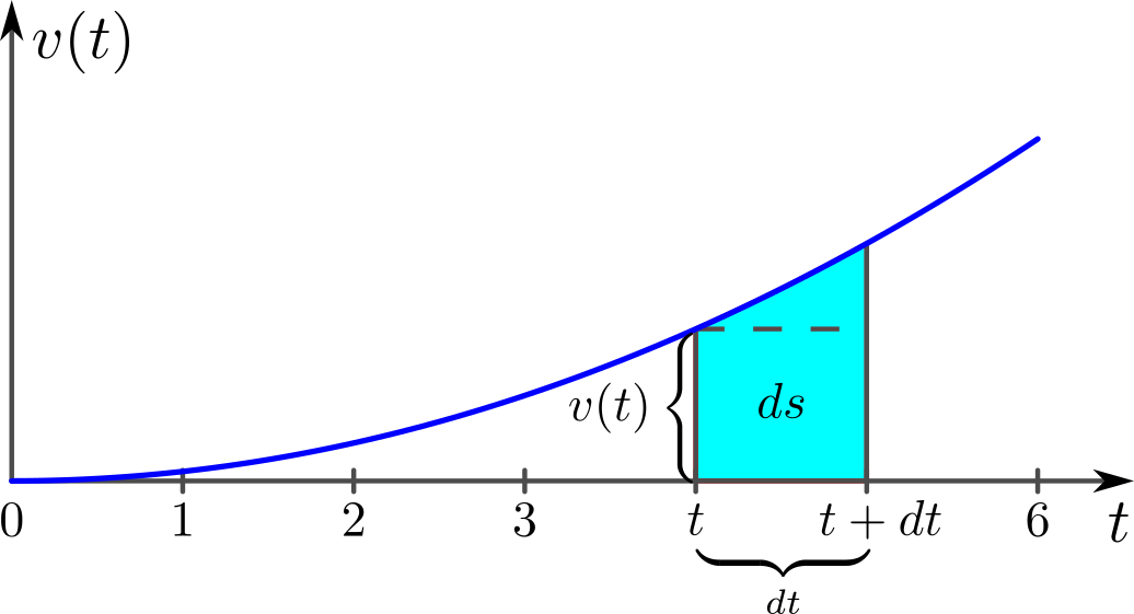 Luas area dibawah kurva/fungsi kecepatan menunjukkan jarak yang ditempuh. Misalkan kita berada pada kemudian kita mengubah nilai sebesar . Tinggi menunjukkan kecepatan. Perubahan pada luas area dibawah kurva disebut . Saat sangat kecil kita bisa menghiraukan luas segitiga di atas. Jadi . Bisa diubah menjadi:


 Secara intuisi seharusnya berlaku: